FACEBOOK LIKES- HOW DOES IT AFFECT THE RECIPIENT’S BEHAVIOR?

FACEBOOK LIKES- HOW DOES IT AFFECT THE RECIPIENT’S BEHAVIOR?

In this post, I am going to share the findings of a recent research by Facebook AI research team in the paper titled “Attitudes and Behaviors around receiving Likes on Facebook” by Scissors et. al. published in CSCW’16 held at San Francisco, CA. In this paper, they have dug deep into how likes affect people with varying mindsets and personalities and what matters more to them- the number of likes or from whom the likes have come from. They also have tried to find out the minimum number of likes with which a person feels content and what affects this number? This number has not been precisely found yet, still most people are content with 1 or 2 likes. They have also discussed a phenomenon called as like paradox, a corollary of friendship paradox- it finds out that a person’s friends has more number of likes on an average than the person himself or herself and this is mainly because the person’s friends have more friends than the person himself or herself. Lightweight, one-click feedback actions occur on Twitter, Flickr, Google Plus, and many other platforms. We focus on Facebook Likes because of the site’s size and scope. Roughly half (44%) of Facebook users Like content posted by their friends at least once a day , generating around 4.5 billion Likes daily as of 2013 . In addition, for some people, “getting feedback on content you have posted” is a major reason for using Facebook . Because a Like takes only one click to produce, it may be an easy way for acquaintances and more distant friends to maintain relationships without requiring a lot of effort or context. On the other hand, Likes may be perceived as less meaningful than comments or posts directly on friends’ walls. Despite being a less effortful form of communication than comments or messages, we view Likes as social cues that send a signal both to the person who created the post as well as to the poster’s network of friends. Given the ubiquity of Likes on Facebook, their theoretical importance as a social grooming tool [9], and this ambiguity around their significance, it is important to understand the value people ascribe to Likes so that we can better understand . motivations for sharing and the role of lightweight feedback in the social media ecosystem.

Methodology of Research and Results:-

Participants:-

Survey participants (N = 2,109; 56% female; ages 13 to 90, mean = 40.3) were recruited through a banner on Facebook displayed to English speakers in the U.S. who had a Facebook account for at least 12 weeks, posted any type of content at least twice, and received at least two Likes in the past 12 weeks. Since the questionnaire focused largely on the experiences of receiving Likes on one’s posts, we first asked participants how often they post to Facebook. Five percent (N = 114) of participants reported that they never post to Facebook and thus were excluded from analyses, leaving a sample of N = 1,996. Participants had an average of 491 friends (min = 1, max = 4,912) and had been using Facebook for 5.9 years (min = 97 days, max = 11 years). During the 28 days prior to the survey, participants logged in to Facebook on an average of 27.4 days (min = 2, max = 28). Compared to a random sample of US, English-speaking Facebook users, our sample was about 3 years older, had 13% more friends, was active on Facebook 2 more days out of the previous 28, and had a Facebook account for 9 months longer on average (all p’s < 0.05). Our sample had 3.5% more women. There was no significant difference in Likes received per post between our respondents and the random sample (M = 18.2 vs. M = 17.8, p = 0.06).

Behavioral data:-

Survey responses were matched to behavioral data from Facebook’s server logs for the prior 12 weeks. All data was de-identified and analyzed in aggregate by Facebook employees. Behavioral data included the number of posts, number of Likes and comments given and received, and the average number of Likes and comments received per post across participants’ 970,135 friends

Procedure:-

Participants filled out an online survey with two sections:

( 1)   attitudes and behaviors about Likes on Facebook and  

( 2)   personal characteristics; sections were presented in counterbalanced order

Items were measured on a 5-point Likert scale (1 = strongly disagree to 5 = strongly agree) unless otherwise indicated.

Measures:-

Self-esteem: Participants completed the 10-item Rosenberg self-esteem scale , which included items like “On the whole, I am satisfied with myself,” and “I take a positive attitude toward myself” (M = 4.14, SD = .85, α = .91).

Self-monitoring: Participants completed a modified version of the self-monitoring scale . The four items participants completed were: “When I am uncertain how to act in a social situation, I look to the behavior of others for cues”; “At parties I usually try to behave in a manner that makes me fit in”; “I try to pay attention to the reactions of others to my behavior in order to avoid being out of place”; “If I am the least bit uncertain as to how to act in a social situation, I look to the behavior of others for cues.” (M = 3.06, SD = 1.02, α = .85).

Extraversion: Several studies have previously investigated the role of extraversion and Facebook use, including its role in group membership and its relationship with self-monitoring . Therefore, we also included a measure of extraversion in this study. Participants completed the four extraversion questions from the Big Five personality scale [6] (M = 3.22, SD = 1.01, α = .82).

Relationship Maintenance Behaviors: Participants filled out the Facebook Relationship Maintenance Behaviors scale [9]. Example items: “When I see a friend or acquaintance sharing bad news on Facebook, I try to respond” (M = 3.94, SD = .78, α = .81).

Attitudes and Behaviors about Likes

We asked people a series of questions related to their experiences with Likes on Facebook:

•   “How often do you post on Facebook (e.g., status update, photo, video, link)?” (1 = never, 5 = multiple times a day)

•   “Why do you think people ‘Like’ your posts?” (open-ended)

•   “If my post does not receive enough Likes, it makes me feel bad” (5pt agreement scale)

•   “There are certain people whose Likes I care about more than others.” (5pt agreement scale)

•   “On average, how many Likes do your posts get compared to your friends' posts?” (1 = my posts get far fewer Likes, 3 = our posts get about the same number of Likes, 5 = my posts get far more Likes)

“Which is usually more important to you, the number of Likes you get or which people Like your posts?” (1 = The number of Likes I get is much more important, 3 = They're both equally important, 5 = The people who Like my posts is much more important)

•   “In general, how much do you care about receiving Likes from the following types of people?” (random order:

Parents; Family members other than my parents; Close friends; Coworkers; Acquaintances; My spouse, romantic partner, or love interest; A former romantic partner; My manager, teacher, or supervisor; Potential employers or professional contacts; People I don't know).

Finally, we asked three questions about receiving “enough” Likes per post:

•   “If one of your posts were to get ‘enough’ Likes, how many Likes would that be? Please write in a number below.”

•  “How did you arrive at that number?” (open-ended)

•   “How important is it for you to get ‘enough’ Likes on your posts?” (1 = not at all important to 5 = extremely important)

RESULTS:-

In the 12 weeks prior to taking the survey, the median participant made 5.25 posts per week (mean = 11.8), “Posts” include photos, text, links, check-ins, and re- shares; multi -photo posts were batched and counted as a single post. The median person received 12.8 Likes per post (min = 0.07, mean = 18.2, max = 692.1). Figure below shows the 12-week averages for all participants.

        

                            FIG 1:AVERAGE LIKES RECEIVED PER POST

                                            FIG. 1: -  AVERAGE LIKES RECEIVED PER POST

About half (52.7%) of participants said that getting “enough” Likes was important to some extent. Yet only 16% of participants agreed with the statement “If my post does not receive enough Likes, it makes me feel bad.” Though most respondents did not feel badly about not getting enough Likes, in open-ended responses they noted they think their friends Like their posts for a number of self-affirming reasons including agreement, attention, supportiveness and empathy.

How many Likes are enough?

Participants proposed a wide range of values for “enough” Likes per post, with the median person volunteering that 8 Likes was “enough” (see Figure 2; numbers larger than 500 were omitted, excluding 3.4% of the sample from that question). Roughly ¼ of respondents reported that 1 or 2 Likes was enough, commenting in open- ended responses that they wanted to be sure someone had seen their posts (e.g., “If it gets at least one or two likes, then I know someone saw it, and that is good enough for me." and “If my post can impact at least one person then I'm happy.”). Beyond 1-2 Likes, people had a variety of reasons for the numbers they chose:

Do people receive “enough” Likes per post?

Roughly two-thirds (62.5%) of participants received what they consider to be “enough” Likes per post in the previous 12 weeks (see Figure 3). Of the remaining third, they fell short by an average of 27.9 Likes (median = 8.9). (Note that this statistic omits 3.4% of respondents who had values greater than 500 for “enough.”) But only some people care about Likes. When removing participants who said they did not care “at all” about receiving enough Likes, 49.9% of participants received what they consider to be “enough” Likes per post, with the average person receiving 6.5 more likes than his or her threshold, and the median person receiving exactly enough (a difference of 0.04 Likes per post). For those who felt they didn’t receive “enough” Likes, what might have led to their inflated expectations? One factor may be the Like paradox as per their research.

FIG. 2: RESPONSES TO ENOUGH LIKES PER  POST                      FIG. 3: AVERAGE LIKES RECEIVED PER POST                                                                                                                  POST BY RESPONSES TO ENOUGH  LIKES PER POST             

                                                             

The Like Paradox

Similar to the friendship paradox, where most people have fewer friends than their friends have [12], in this work we demonstrate a “Like paradox:” people receive fewer Likes on their posts than their friends get. During the 12 weeks prior to the survey, participants’ friends received roughly twice as many Likes per post (median = 23.8) as they did (median = 12.8). Figure 4 shows the difference between the two. Why did their friends receive more Likes? Those friends had roughly twice as many friends as our participants (see Figure 5).

Only some participants perceived this discrepancy in Likes between themselves and their friends: 28% reported on the survey receiving fewer Likes than their friends and 56% thought they got about the same number of Likes. This suggests that there may be other factors that influence people’s impressions of the number of Likes they should receive, not just how many their friends receive.

                                                                                          

                      

FIG. 4: AVERAGE LIKES RECEIVED BY                                                          FIG. 5:  FRIENDSHIP PARADOX

SURVEY RESPONDENTS AND THEIR FRIENDS.

Who do people want Likes from?

Participants most wanted to receive Likes from close friends (73% “want” or “really want”), romantic partners (60%), and family other than parents (50%) (see Figure 6). On the other hand, people least want to receive Likes from people they don’t know (34%), potential employers or professional contacts (25%), and managers/teachers/ supervisors (24%).

Individual differences in caring about Likes

There are a number of psychological traits that influence the extent to which people care about getting Likes on Facebook. Table 1 shows three regressions estimating responses to three survey questions about (1) the importance of getting enough Likes, (2) whether people feel bad if they don’t receive enough Likes, and (3) whether they think they receive more Likes than their friends.

All three models control for age, gender, friend count, and the number of days in the past month the participant logged in to Facebook. Each model includes self -esteem, self-monitoring, extraversion, and Facebook relationship maintenance behaviors. Correlation between the scales was low (max r = .37 between extraversion and self- esteem). The third regression includes an additional binary variable indicating whether a person actually received more Likes per post than his or her friends. All continuous independent variables except for age were standardized (age was only centered), and friend count was logged base 2 to control for skew and then standardized.

 

    FIG. 6: PREFERENCES FOR LIKES FROM DIFFERENT TYPES OF FACEBOOK FRIENDS.

	Importance of getting		Feel bad if don’t get		Perception of # Likes
					received compared to
	enough Likes		enough Likes
					friends
Variable	β	SE	β	SE	β	SE
Intercept	1.90 **	.03	2.12**	.03	−.23 **	.03
Self-esteem	−.14**	.03	−.23**	.03	.09 **	.02
Self-monitoring	.20 **	.02	.28**	.03	.02	.02
Extraversion	−.01	.03	−.05	.03	.16 **	.02
FB Relationship Maintenance	.09 **	.03	−.02	.03	.05 *	.02
Age	−.00	.00	−.00	.00	.01 **	.00
Gender	.09	.05	−.00	.05	−.02	.04
Friend Count (Log2)	.18 **	.03	.10**	.03	.20 **	.02
# of days logged in over the	−.04	.02	.01	.03	.07 **	.02
past month
Friends receive more Likes per					.27 **	.05
post
Adj. R-squared	.09		.12		.19

N = 1996; * = p < .01, ** = p < .001

Table 1. Models predicting (1) importance of getting enough Likes, (2) feeling bad about not getting enough Likes, and (3) perception of the # of Likes received compared to friends’ Likes received.

DISCUSSSIONS:

about half of participants reported that they did care to some extent about getting enough Likes, suggesting that the number of Likes may be more important if a certain minimum is not met. Of the people who cared about getting enough Likes, about half of them received more than enough, while the other half received too few by their standards. When asked how many Likes was “enough”, people tended to have a rationale for this number, which was higher than their typical number of Likes by about 9 Likes. This is possibly due to the Like paradox whereby one’s friends get more Likes than one does, or the feed ranking algorithm showing people content that receives a lot of Likes.  The finding that some people are not getting what they consider to be enough Likes on their posts has implications for Facebook in particular, and for SNSs more generally. For instance, the pressure to get enough Likes that some people feel could be reduced by providing other social cues. This could be through development of alternative one-click actions that aren’t public-facing, or signals such as “read receipts” to provide more insight to audience composition. The pressure to get enough Likes could be also be reduced by encouraging people to share with specific subsets of friends, like in a closed group or on a specific friend’s wall. Alternatively, other SNSs have addressed their versions of the Friend paradox and/or Like paradox in other ways. For example, Snapchat does not show the amount of feedback on others’ content and feedback is provided in other ways (namely, content production of one’s own). The authors have also shown that self-esteem, self-monitoring, and engaging in relationship maintenance behaviors were all related to perceptions and attitudes about Likes.

REFERENCE:

For further reading, you may refer the paper “What’s in a Like? Attitudes and behaviors around receiving Likes on Facebook” by Lauren Scissors, Moira Burke, Steven Wengrovitz .web link

Fraud Detection in Online Reviews by Network Effects

Veracity means the quality of being truthful or honest. Now, as the internet grows in volume as well as importance, the importance of reviews and comments is gradually increasing, specially in field of eCommerce. Deception in reviews influences the customers as it gives fake information about the product on which they are dependent. As well as in this competition era, competitors write fake reviews to defame the product or services of their competitor. That's why it is important to detect the Veracity in the reviews.
But data-set is growing linearly with time, hence form a complex network.

Fraudeagle,  is the network based approach to tackle the opinion fraud detection. 

Problem Description: 
Consider the problem of spotting fraudulent reviewers, and consequently spotting fake reviews in online review datasets.

For eCommerce, Online review datasets consists of :

(1) Reviewer -  {'Fraud','Honest'}

(2) Product    -  {'Good','Bad'}

(3) Reviews   -  {'Positive','Negative'}

Reviewer is Honest if s/he writes mostly Positive review for Good product and Negative review for Bad product. and vice-versa for Fraud reviewer.
Figure 1 showing the Signed Bipartite Graph, where nodes are product and user(reviewer) and edges are signed as positive (+ / thumbs up) if rating is above threshold, otherwise negative (- / thumbs down).

Users 1-4 are honest while 5-6 are fraud, and Products 1-2 are good quality while 3-4 are bad.
The network structure and the sentiment (sign) of edges are observed. The fraudsters write fake reviews for the products except the + review from user 6 to product 2.

The goal is to develop a method to automatically label the users, products, and reviews in the large complex network.

Problem Formulation:
signed Inference Algorithm (sIA): Given a signed network G (V,E).

• User set U={u₁, u₂, ..., u_n} and Product set P={p₁, p₂, ..., p_m} are linked with edge e(u_i, p_j, s) ∈ E, s ∈ {+,-}.
• U∪P=V.
• Each node in V and each edge in E is a random variable that takes a value from an appropriate label domain.
• L_U = {honest, fraud}, L_P = {good, bad}, and L_E = {real, fake}. 
• In this classification task,
• let Y_V = Y_U ∪ Y_P and Y_E respectively denote the nodes and edges the values of which need to be assigned, and let y_i refer to Y_i’s label.
• Let Ψ denote a set of clique potentials that consists of two types of functions:
•  For each Y_i ∈ Y_U and Y_j ∈ Y_P , ψ_i ∈ ψ is a prior mapping ψ^U_i : L_U → R ≥0, and ψ^P_j : L_P → R ≥0, respectively
• For each e(Y^U_i, Y^P_j, s) ∈ E, ψ^s_ij ∈ Ψ is a compatibility mapping ψ^s_ij : L_U × L_P → R ≥0

Given an assignment y to all the unobserved variables Y^V and x to observed ones X^V (variables with known values), our objective is to maximize the probability distribution

Given,

- a bipartite network G = (V, E) of users and products connected with signed edges,

- prior knowledge (probabilities) of network objects belonging to each class, and

- compatibility of two objects with a given pair of labels being connected.

Now, Score the graph by Fraudeagle Scoring in Step 1 and then obtain induced subgraph and apply clustering algorithm to partition as apply in step 2.

(I) Scoring for fraud detection (Convergence algorithm) :

Proceeds by making each set of Y_i ∈ Y_U and Y_j ∈ Y_P alternately communicate messages with its neighbors in an iterative fashion until the messages stabilize, i.e. convergence. After they stabilize, calculate the marginal probabilities; say of assigning Y_i with label y_i by computing the final belief b_i(y_i).

where m_i→j is a message sent by user Y_i to product Y_j (a similar equation can be written for messages from products to users), and b_i(y_i) denotes the belief of user i having label y_i (again, a similar equation can be written for beliefs of products). α’s are the normalization constants, which respectively ensure that each message and each set of marginal probabilities sum to 1.

The prior beliefs ψ^U_iand ψ^P_j, respectively of users and products can be suitably initialized if there is any prior knowledge of the objects.

(II) Grouping for analysis and sensemaking (Clustering Algorithm):

• Project the top users back on the review graph, and obtain the induced subgraph including these users along with the union of products that they rated. Then partition this subgraph into clusters to gain more insight about how they are organized in the network.

• For partitioning, can use any graph clustering algorithm: Cross-associations (CA) clustering algorithm on the adjacency matrix of the induced graph performs clustering by finding a permutation of the rows (users) and columns (products) of the matrix such that the resulting matrix contains homogeneous blocks (defined by the clustering), where dense blocks correspond to near-bipartite cores (e.g., a team of users attacking on a target set of products).

Lemma 1 Proposed Fraudeagle is scalable to large data (complex graph), with computational complexity linear in network size. 

STEP 1 Time complexity O(|E|d²t), 

where |E| is number of edges in the network,d is maximum domain size of variable(i.e. number of classes), t is the number of iterations until convergence.

STEP 2 Cluster the induced graph on top users and their products using the CA algorithm, which is also linear in number of edges. The induced graph is also much smaller than the input graph.

References: Opinion Fraud Detection by Network Effects, review spam detection, Review Graph based Spammer Detection  

Marvel Universe looks almost like a real social network

Collaboration networks have always been an active area of research in social networks. You must have heard about the Movie Actors network, scientific collaboration networks, etc. but have you ever heard of the Marvel Universe collaboration network? It is an artificial network of Marvel Comics characters but mimics a very real-life networks behavior. In this network, the nodes correspond to Marvel Comics characters, and there exists an edge between two characters if they have jointly appeared in the same Marvel comic book. The joint appearance of the pairs of characters in the same comic book allows us to form a collaboration network for the Marvel Universe network.

The Marvel Universe network

The Marvel Universe network (MU) has nodes that are popular Marvel characters and two characters are linked when they jointly appear in a significant way in the same comic book. The data set used was the Marvel Chronology Project (MCP) that collects over 96,000 appearances by more than 6,000 characters in about 13,000 comic books.

Analysis of the network

Initially, a bipartite graph(X, Y, E) where nodes X correspond to Marvel characters and nodes Y correspond to the comic books, and edges from every character to all the books where it has appeared, is generated. A collaboration network, called as the MU network,  is then derived from this bipartite graph as its projection on its set of characters.

Basic data on appearances of characters in comic books

Number of characters:	6,486
Number of books:	12,942
Mean books per character:	14.9
Mean characters per book:	7.47

The bipartite graph

Let Pb(k) represents the probability that a comic book has k characters appearing in it, and Pc(k) represents the probability that a character appears in k comic books. 
It was found that Pb(k) follows the power-law tail represented in Fig. 1

Fig.1. Probability Distribution Pb(k)

The distribution of Pc(k) obtained here is normally not find in bipartite graphs associated with collaboration networks,

Fig.2. Probability Distribution Pc(k)

The exponent value is much smaller than other values for similar collaboration networks, that usually ranges from 2 to 3.

The null random model

The study starts with a random bipartite graph, called MU-BR graph hereafter, with 6,486 nodes-characters and 12,942 nodes-books, and whose edges have been created using the same distributions Pc(k) and Pb(k) of outgoing and ingoing edges found above. Then, a projection of this random graph called as the MU-R graph was generated where the nodes correspond to characters and its links represent to be connected to the same book in a MU-BR graph.

Summary of results of the analysis of the MU network.

Mean partners per character:	51.88
Size of giant component:	6,449 (99.42%)
Mean distance:	2.63
Maximum distance:	5
Clustering coefficient:	0.012

Distribution of partners:

Separation

Here the research tries to relate the MU network to the mathematicians’ collaboration network and see if there exists someone like Erdos. The diameter found in the MU network is 5 implying there is always a chain of at most 4 collaborators connecting any two connectable characters in the Marvel Universe. Finally, it tries to find out a Marvel character who is like Erdos sitting at the center of the the giant component, one that minimizes the total distance from it to all other nodes in the network and it turns out the character is the Captain America, who is, on average, at distance 1.70 to every other character in the network.

Clustering coefficient

The popular collaboration networks having studied so far have large clustering coefficients in general for most social networks. The low value of the average distance between connected nodes and this large clustering coefficient taken together is defined as the small-world networks. Against what happens with real-life social networks, it turns out that the clustering coefficient of MU is small. Its value is CMarvel = 0.012, while the clustering coefficient of a random network with 6,486 nodes and 1,68,267 links is Crandom = 0.008 which implies CMarvel is roughly 1.5 × Crandom, and not several orders of magnitude larger which separates it from the real-life, collaboration networks.

Degree Distribution P(k)

The degree distribution is yet another interesting statistical feature that can help differentiate random networks from non-random networks. A random network with n nodes and m links follows the binomial distribution

 

where p is given as,

On the other hand, the collaboration networks in general follow the distribution which has a heavy tail represented by either a power law as

for some positive constant τ,  or a power law form with an exponential cutoff as

where τ and c are positive constants, and c is large.

The data for the MU network fits a power law distribution with an exponential cutoff and the distribution was represented as

Thus, the degree distribution of the MU network has a power law tail with cutoff as can be seen in Fig.3. A smaller value of  τ say less than 2 represents the domination of the MU network properties by the few actors with a large number of collaborators which is quite similar to many real-life networks. On the other hand, the value of τ much smaller than 2 shows that the weight of characters like Captain America, Spider-Man, and other major -heroes is very large that what happens in real life networks like scientific or any other collaborator networks and this is expected as there are no super-heroes in real life.

 Fig.3. Probability distribution P(k)

Conclusions

The article thus realizes that though to some extent the MU tries to mimic real-life networks, and it is largely different from a random network, but it cannot hide its artificial origins completely.

For more details have a look at http://arxiv.org/pdf/cond-mat/0202174v1.pdf

Centrality measure to find the Importance of Nodes in dynamic Networks

There has been a lot of work done in defining different metrics able to characterize the importance of nodes in networks. Among them, centrality measures have proved to be pertinent as they relate the position of a node in the structure to its ability to diffuse an information efficiently.There is no investigation regarding the fact that the network structure evolves and that node importance may evolve accordingly.
Most centrality measures are based on the study of paths in the network: a node will be important for instance if the paths from it to other nodes are short, or if it lies on shortest paths between many pairs of nodes. One motivation for this is that links can act as a dissemination medium for some phenomena occurring on the network. For instance individuals can exchange information when they communicate, or a message can be forwarded from computer to computer until it reaches its destination.It has been acknowledged for some time that networks are dynamic in nature: nodes and links come and go with time.In the case of centrality, some works have been concerned with efficiently updating the centrality values of the nodes when a change occurs in the network. In many cases however, the time scale at which the network evolves is the same as the one at which a dissemination phenomena may occur on the network. This is the case for instance when a disease propagates among individuals when they are in contact, or when an information is disseminated by email messages.

A small example of a dynamic network

Here the paths change during the network time span, and thus the importance of nodes varies. Consider the toy example of Figure. This small network composed of five nodes evolves during four distinct time steps. One can see that, intuitively, the importance of node b is much stronger at time t = 1 than at time t = 3. Indeed, at time t = 1 it forms a bridge between node a and nodes c, d and e, thanks to the links that exist at time t = 2.
Here we explore a natural extension of the closeness centrality to the case where paths may start at any time during the network’s time span. This temporal closeness characterizes the importance of any node at any given time. We study two datasets and observe that:

• node importance does vary with time, and therefore capturing the global importance of a node with an aggregate value might be misleading
• in some cases the dynamic of the network is such that it is meaningless to identify nodes more important than others; in other cases, temporal closeness may help identifying a node consistently important for the whole network time span

A dynamic network G = (V,E) consists of a set V of nodes 1 and a set E of timed links of the form (u, v, t) where u, v € V and t is a timestamp. Throughout the paper we consider networks as undirected, i.e. a link (u, v, t) is equivalent to a link (v, u, t).A temporal path in a dynamic network consists of:

• for all i, i = 0..k − 1, ui+1 = vi
• for all i, i = 0..k − 1, ti < ti+1.
• t0 >= ts

We say that such a path is a path from  u0 to vk starting at time ts. Its duration is equal to tk − ts. We will say that a path from u to v starting at time ts is a shortest path if it has the least duration among all paths from u to v starting at time ts. We define the distance from u to v at time t to be the duration of a shortest path from u to v starting at time t, and we denote it by dt(u, v). If there is no path from u to v starting at time t, we consider that dt(u, v) = infinity.For example, in the dynamic network of Figure, there are two temporal paths from e to b starting at time t = 2. The first one consists of the single link (e, b, 2), and its duration is 0; the second one consists of the links (e, d, 3) and (d, b, 4) and its duration is 2. The temporal distance from e to b at time 2 is therefore d₂(e, b) = 0. Note that the temporal distance from e to b at time 1 is d₁(e, b) = 1: the temporal shortest path has the same link sequence than the one starting at t = 2 (it is the single link (e, b, 2)), but the starting time is different. Since there is no temporal path from c to e starting at time t = 3, d₃(c, e) = infinity.

Several variants have been introduced in the literature, most notably concerning the constraint ti < ti+1.Some variants weaken it to ti <= ti+1, while others strengthen it to ti <=ti+1 +(delta), where _ is a parameter representing the time needed to send a message along a link. The relevance of these variants depends on the context.Preliminary work shows that this has little influence on the results.

We recall that the closeness of a node u in a non-evolving network is defined as:

The average of the closeness of all nodes has been defined as network efficiency.

Though some extensions of the closeness have been defined for the case of dynamic networks, their goal is not to take fully into account the fact that temporal distances vary according to the paths’ starting time. We therefore here define the temporal closeness of a node u at time t as:

and we define the temporal efficiency Et(G) of network G as the average over all nodes of the temporal closeness at time t.

Building upon this notion of efficiency, we can study another metric that quantifies the impact a node has on a network. The notion of delta-centrality characterizes how much a given node (or group of nodes) impacts the efficiency. It is defined as the relative change of the network efficiency when the considered node (or group of node) is removed from the network. Following this, we study the extension of the delta centrality to the dynamic case. The temporal delta-centrality of a node v at time t is defined by:

where G\v is the network obtained from G by removing node v and all its adjacent links.

In order to study the behaviors of the metrics introduced above, we study two datasets that present different characteristics and come from two very different contexts:

• Rollernet: this dataset was collected during a rollerblade tour in Paris in August 2006. The tour is a weekly event and gathers approximately 2500 participants. Among these, 62 were equipped with wireless sensors recording when they are at a communication distance from one another. The dataset therefore contains the proximity links between the persons carrying the sensors. The total dataset duration is approximately 2 hours and 45 minutes.
• Enron: this dataset contains the 252 759 emails that 151 Enron employees exchanged during three years. It records information on the senders, receivers, and the moment they were sent. Note that by nature, the links are directed but for a fair comparison with the Rollernet dataset, we treated them as undirected in the present study.

A) Temporal efficiency and temporal closeness over time:

Above Figure presents the time evolution of the temporal efficiency for each dataset. We can see that the value fluctuates widely for both of them. Notice that for Enron, even though it fluctuates, the efficiency tends to increase with time 3. This is caused by the fact that, as shown previously, the number of pairs that are reachable from one another increases with time throughout the dataset duration. The final collapse stems from the fact that, towards the end of the dataset, less and less temporal paths exist.We expect that these fluctuations in the efficiency will impact the individual node’s closeness.

Observations can be summarized as follows:

• Node importance varies with time: a given node may be very important at one time, and not so important at another time; therefore it is not relevant to consider only aggregate values that summarize the importance of nodes on the whole network time span.
• Different datasets have different properties regarding node importance; for one of our datasets, the importance of all nodes fluctuates extremely rapidly between high and low values; it is meaningless in this case to state that one node is more important than another, except for a very limited time span; for our other dataset however, we find that some nodes are consistently important (or unimportant) for the whole network time span.

The Power of Consensus: Random Graphs Have No Communities

Communities are a powerful tool to describe the structure of complex networks. Algorithms aiming at maximizing a quality function called modularity have been shown to effectively compute the community structure.
However, some problems remain:
It is possible to find high modularity partitions in graph without any community structure, in particular random graphs.
In this article i will state the notion of consensual communities and show that they do not exist in random graphs.
For that, we exhibit a phase transition based on the strength of consensus:
below a given threshold, all the nodes belongs to the same consensual community 
above this threshold, each node is in its own consensual community.

In random graphs, however, links appear independently of each other, so a strong inhomogeneity in the density of links on these graphs is not expected. Therefore, random graphs should not have communities using the previous definition.
It is however possible to find partitions with significantly high modularity in random networks.
A good community detection algorithm should therefore be able to find communities but also to indicate their absence.
Author of the paper (The Power of Consensus: Random Graphs Have No Communities) has proved that random graphs only contain trivial consensual community, i.e. containing all the nodes of the graph or only a single node. and also showed there is a phase transition between these two states depending on a resolution parameter.

In random graphs, all pairs of nodes have the same probability to be connected. Hence, they should not have preferential binding inducing specific and identifiable nodes groups.
Therefore, we could conclude that there are no community structure in random graphs.
However, several studies show that it is possible to find partitions with high modularity in random graphs [ref1], [ref2]

Indeed, the links concentration fluctuates in generated graphs, which means that subsets of nodes with a density larger than global density can appear.
The phenomenon is even more pronounced in regular or quasi-regular graphs, like trees, torus or grid graphs, in which community detection algorithms can also find partitions with good modularity

A good algorithm for community detection should indicate that communities obtained in random graphs are not real  communities. We will now show that random graphs do not exhibit any non-trivial ccs. For this, 

we will use random graphs model: the classical Erdos-Renyi model 

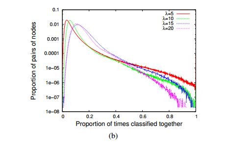
Above figures shows Distribution of the pij(he probability for drawing an edge between two arbitrary vertices ) averaged over 100 random Erdos-Renyi  graphs.

(a) Networks with different number of nodes n and an average degree of λ = 20.

(b) Networks with n = 1,000 nodes and different values of the average degree.

This concentration of values implies that even if partitions with a good modularity can be found in random graphs, these partitions are very different from one another since most pairs are classified in the same community only once every ten runs

 "Comparison with Real Graphs"

 
To compare more precisely real and random networks, they generated random graphs from the Erdos-Renyi model that have the same size and the same average degree (resp. the same degree distribution) as two realworld networks.

Fig 2: pij distribution for two real-world networks together with Erdos- ˝ Renyi ´ and configuration model random graphs with the same size: the email network (top) and the collaboration network (bottom)

In Fig 2., the Erdos-Renyi  model shows no pair of nodes with pij = 0, which means that all pairs of nodes have been grouped together at least once during 1,000 runs of the Louvain algorithm, regardless of their position in the network.

Conversely, there is nearly no pair of nodes which are always grouped together, except for the leaves (nodes of degree 1) of the network which are always grouped with their only neighbor. This presence of nodes of degree 1 is very common

There is two direct consequences of this distribution: 

(i) for very low values of the threshold, there is a single CC containing all nodes since there is no value close to zero and therefore the virtual graph contains all links, and

(ii) for large values of the threshold, the virtual graph contains almost no links and therefore high threshold CCs are reduced to single nodes.

                           Fig 3. Proportion of internal links for a random graph with 10,000 nodes

Finally, we can compute the value of this threshold. 

Let us assume that k% of links are intra-community links. Then, this means that for each execution of the algorithm, one node u will be put in expectation with k% of its neighbors, or equivalently each neighbor will be with the given node u for k% of the executions. This value k is thus the value of pij corresponding to the p that we have used so far. Computing exactly the value of p is an open problem that seems to be difficult [ref2]. However, numerical studies (see Fig. 3) show that it decreases with the graph density but that the exact decrease pattern is quite complex.

It would be interesting to analyze this phenomenon on others random graphs families such as Watts-Strogatz model,Barabasi-Albert model, etc.

On a more general perspective, the computational issue has to be addressed. Indeed, computing ccs on large graphs can be hard even with very fast underlying algorithms such as Louvain, and different techniques should be used, such as local computations for instance.

Also, to show the above behavior, i had simulated the following in R :

First, we will generate one random graph according to the Erdos-Renyi model

# Generate random graphs according to the Erdos-Renyi model

 graph <- erdos.renyi.game(50, 0.3, type=c("gnp", "gnm"),              directed = FALSE, loops = FALSE)

then , we will apply cluster_walktrap function for detecting Community strucure via short random walks in r on the graph. and observe the community patterns generated and No. of steps(iteration) of algorithm.(R code is as below :)

## no of steps we are going to perform of algorithm  cluster_walktrap
## cluster_walktrap is function for Community strucure via short random walks in r
allsteps <- 1:10 

##stores all the membership vectors for membership of particular node of graph
membershipframe <- 1:50 

##stores modularity values for each iteration.
m <- c() 

for (i in allsteps ){
    wtc <- cluster_walktrap(graph,steps = i) ##find community by "i" steps of "cluster_walktrap"
    m<- c(m,modularity(wtc)) ##store modularity
    membershipframe <- cbind(membershipframe,membership(wtc)) ##store membership
    ##save plots
plotname <- paste("rplot",i)
    plotname <- paste(plotname,".jpg",collapse = "")
    jpeg(plotname)
    plot(wtc,graph)
    dev.off()
}

all the plots are looking like :

From this experiment on small graph of 50 vertex, we can get intuitive idea o, what author is trying to say from FIg.2. and we can see after each step, how nodes are merged.

References : [mainref]  , [ref1] , [ref2]